Medium Quick Review of the Best Networks Cnn

Review On Faster RCNN

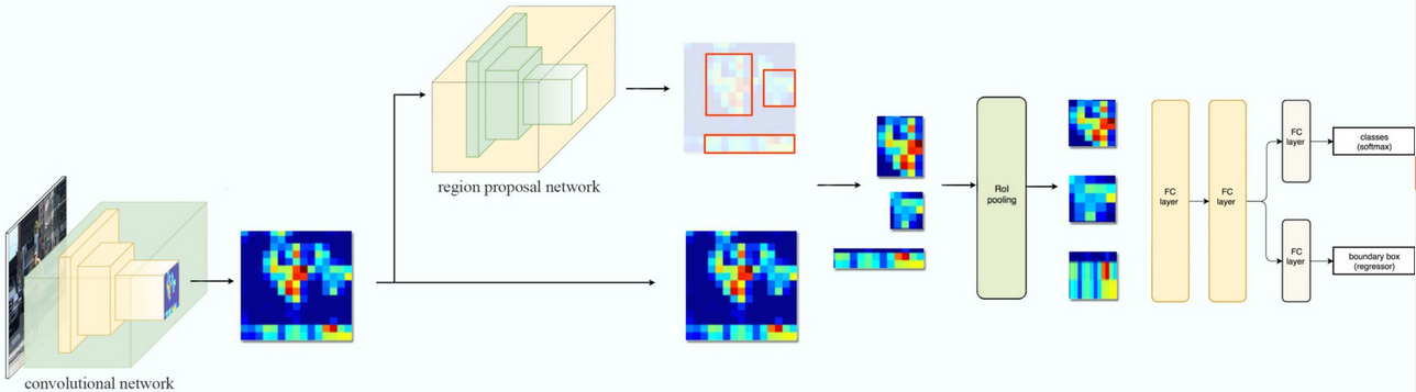
In this article we will review faster RCNN paper by Shaoqing Ren, Kaiming He, Ross Girshick, and Jian Sunday. Before reading this article I would recommend anybody to become through the fast RCNN review if interested.It helps to understand the concepts better. Compared to other region based networks faster RCNN uses the same network for region proposals and object detection.Nosotros will divide the article in to 5 sections

1. Region proposal network

ii. Training

3. Experiments and observations

4. Detection Results

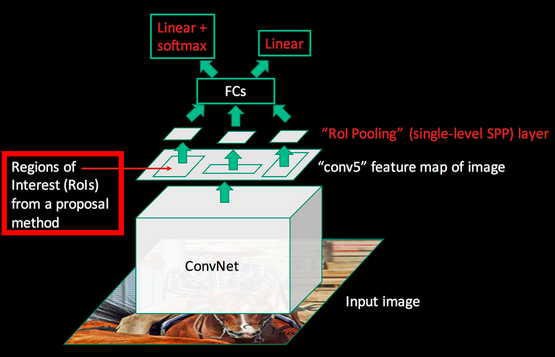
1. Region Proposal Network

In Fast RNN selective search and detection network are decoupled.Merely Decoupling is non a good idea. Say for example, if selective search has simulated negative, this mistake will touch on the detection network directly. Information technology is better to couple them together such that they are correlated to each other.

Earlier explaining about region proposal network it is expert to know, why we need it and what are the short comings of selective search used in RCNN.

Some conditions for replacing selective search:

• Should produce less than 2000 region proposals
• Equally fast every bit selective search or better
• As accurate equally selective search or ameliorate
• Should be able to propose ROI's with different attribute ratio and scale.

Nosotros will talk over some approaches that will try to solve this:

Approach1: Fast RCNN + image pyramid + sliding window on characteristic maps

In this approach nosotros tin can utilize image pyramids and do ROI projects at unlike scales to feature map.Now we can use sliding window technique on characteristic maps.At each sliding window position we tin practise ROI pooling and thus do classification every bit well equally regression.

Disadvantage: This arroyo volition irksome downwardly the network

Approach2: Fast RCNN + characteristic pyramid

We can use feature pyramid to excerpt ROI'southward from feature maps.ie, we will employ boxes of different shapes to extract ROI's. for example we volition use foursquare,tall rectangle and wide rectangle boxes.We will utilise about 9 types of such boxes.

Only even this approach volition create a total of 40x60x9=14400 bboxes with a 40x60 feature map.So this will also slows down the network

Approach3: Fast RCNN + bbox regressor (RPN)

This approach is the core thought which atomic number 82 to region proposal network.Now we will get to know how RPN works?

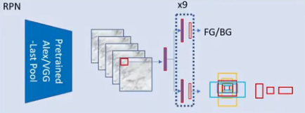
A Region Proposal Network (RPN) takes an image(of any size) as input and outputs a set of rectangular object proposals, each with an objectiveness score. RPN has a regressor (relative regression) every bit well equally a classifier. The classifier will output the probability of predicted ROI as foreground or background.The regressor volition predict (dx,dy,dh,dw) which we add to ROI'due south to lucifer to the ground truth bbox dimensions.

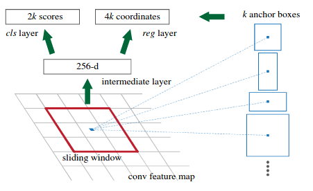
1. The prototype goes through the convolution layers and features are extracted.

ii. Then a sliding window is used for each location over the feature map.

3. For each location nosotros utilize 9 anchor boxes for generating region proposals.we utilise 3 anchor boxes of 3 different scales(128,256,512) and 3 aspect ratios(1:1,1:2,two:1). Thus total of ix anchor boxes.Thus each location generates 9 region proposals.

4. The nomenclature layer outputs 2k scores whether there is object or non for k boxes.

5. The regression layer outputs 4k for the coordinates (box centre coordinates, width and pinnacle) of thousand boxes.

6. With a size of W × H feature map, at that place are WHk anchors in full.

For training RPNs, nosotros assign a binary class label(of existence an FG or BG) to each anchor. We equally-sign a positive label to ii kinds of anchors:

• Anchor/anchors with the highest Intersection-over-Union (IoU) overlap with a footing-truth box

OR

• Anchor that has an IOU overlap higher than 0.7 with ground-truth box.

Note that a single footing-truth box may assign positive labels to multiple anchors.Usually the 2d condition is sufficient to determine the positive samples; merely nosotros notwithstanding prefer the first status for the reason that in some rare cases the second status may discover no positive sample.

• We assign a negative label to a not-positive anchor if its IoU ratio is lower than 0.3 for all basis-truth boxes

With these objective nosotros minimize the following loss function:

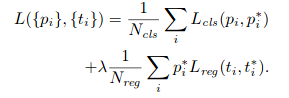
p_i is the predicted probability of ballast i beingness an object.

p_i∗i is the ground_truth characterization which is 1 if the anchor is positive, and 0 if the anchor is negative.

t_i is a vector representing the 4 parameterized coordinates of the predicted bounding box,

t_i∗ is that of the ground-truth box associated with a positive anchor.

The first term is the classification loss over two classes (Foreground or groundwork). The second term is the regression loss of bounding boxes but when in that location is object (i.east. p_i* =1).

The 2 terms are normalized by N_cls and N_reg and weighted by a balancing parameter λ. In our current implementation (every bit in the released code), the cls term is normalized by the mini-batch size (i.east.,N_cls= 256) and the reg term is normalized past the number of anchors locations (i.east.,N_reg∼2,400)

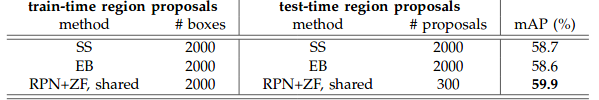
As regions can exist highly overlapped with each other, non-maximum suppression (NMS) is used to reduce the number of proposals from about 6000 to N (N=300)

Now the corresponding locations and bounding boxes volition laissez passer to detection network for detecting the object course and returning the bounding box of that object.

2. Grooming — 4 Step Training

Since the convolution layers are shared the training procedure is quite different:

1. Initialize the RPN network with image net pretrained model. Now train(fine melody) RPN network.

ii. Initialize a seperate detection network with imagenet pretrained model.Now train(fine tune) the split detection network by Fast R-CNN using the proposals generated by the pace-one RPN. At this point the two networks do non share convolutional layers.

3. Nosotros apply the detector network to initialize RPN preparation.In this step nosotros fix the shared convolutional layers and simply fine-tune the layers unique to RPN. We exercise not fine melody the shared convolution layers.

4. Finally, keeping the shared convolutional layers fixed, we fine-tune the unique layers of Fast R-CNN with new ROI proposals from step3.Hither also we do not fine tune the shared convolution layers.

three. Experiments and observations

3.ane Ablation Experiments on RPN

To investigate the performance of RPN network, they conducted several ablation study. Commencement, nosotros show the issue of sharing convolutional layers betwixt the RPN and Fast R-CNN detection network. To practice this, nosotros stop after the second stride in the four-pace training process.

Using separate networks reduces the result slightly to 58.vii% mAP.This is considering in the 3rd step when the detector-tuned features are used to fine-melody the RPN, the proposal quality is improved.Merely With shared conv layers, 59.9% mAP is obtained. And information technology is meliorate than prior arts SS and EB.

3.two λ in Loss Office

We got the all-time results when λ = 10 with VGG16 backbone.

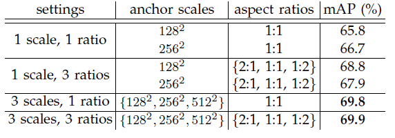
3.3 Scales and ratios

With three scales and 3 ratios, 69.ix% mAP is obtained which is simply lilliputian improvement over that of 3 scales and one ratio. But withal iii scales and iii ratios are used.

three.four Analysis of Retrieve-to-IOU

They likewise computed the recall of proposals at different IoU ratios with ground-truth boxes.Their results are shown in post-obit graphs:

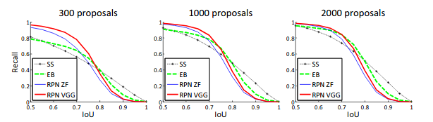
The plots show that the RPN method behaves gracefully when the number of proposals drops from 2000 to 300. This explains why the RPN has a proficient ultimate detection mAP when using every bit few as 300 proposals.

4. Detection Results

four.1 PASCAL VOC 2007

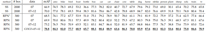
Above tabular array shows the results on PASCAL VOC 2007 examination prepare with Fast R-CNN detectors and VGG-16. For RPN, the train-time proposals for Fast R-CNN are 2000. RPN∗denotes the unsharing characteristic version.

iv.2 PASCAL VOC 2010

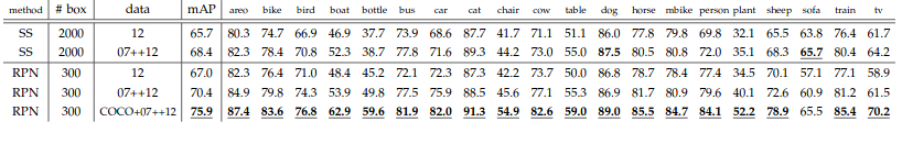
Above table shows the results on PASCAL VOC 2007 examination gear up with Fast R-CNN detectors and VGG-16. For RPN, the train-time proposals for Fast R-CNN are 2000.

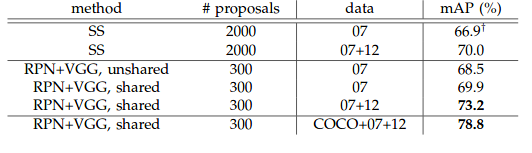
With grooming data using COCO, VOC 2007 (train+val) and VOC 2012 (train+val) dataset, 78.8% mAP is obtained.

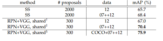
With training data using COCO, VOC 2007 (train+val+examination) and VOC 2012 (railroad train+val) dataset, 75.9% mAP is obtained.

4.iii Detection time

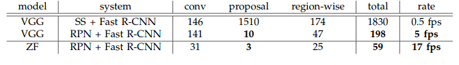
Using SS as RPN and VGGNet as detection network: 0.5 fps / 1830ms
Using VGGNet as RPN and detection network: 5fps / 198ms
Using ZFNet as RPN and detection network: 17fps / 59ms
which is much faster than SS.

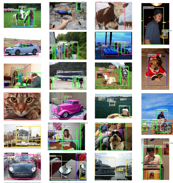
4.4 Some detection examples mentioned in newspaper

Annotation: I did not mention about all the experiments mentioned in newspaper.I only mentioned important ones.y'all tin always refer paper if yous would like to explore more than.

luncefordinet1986.blogspot.com

Source: https://medium.datadriveninvestor.com/a-review-on-faster-rcnn-72d31f50cc52

Share this post